Common Imaging Artefacts

There is no substitute for a high quality image in digital imaging and microscopy
Garbage In gives Garbage Out

Introduction

This webpage illustrates some common artefacts introduced when acquiring images with either not enough contrast (no Koehler illumination), too much or not enough light, out of focus, faint staining, etc. Small details are the first to disappear and images of an inferior quality are the result.
The artefacts shown here ultimately lead to a bias in the results when measurements take place and are a cause of inaccuracy and errors in our research and conclusions.
Proper biological sample preparation, proper use of the microscope and the camera used for image acqusition are the main remedies against these artefacts.

The first part of this webpage shows the relationship between image quality and the segmentation result of the image. The change in detected object shape is shown, compared to a reference image.
The second part of this webpage shows the relationship of the image quality in terms of contrast and the results on feature measurements derived from the image.
The third part of this webpage shows the relationship of the image quality in terms of the dark current of the camera and the influence on ratio measurements.

I. Image quality and segmentation

An image and its histogram

The images above show a digital image and its histogram, which provides us with information about the distribution of the gray-leves of the image. As such it is a very useful source of information about the quality of the image.
The histogram shows two peaks, the one to the left corrsponds with the background, the one on the right corresponds with the foreground.
Definition of a histogram: The histogram of a digital image with gray levels in the range [0,L-1] (eg. 0-255) is a discrete function p(r_k)=n_k/n, where r_k is the kth grray level, n_k is the number of pixels in the image, and k=0,1,2, ... , L-1.
Loosely speaking p(r_k) gives an estimate of the probability of occurrence of gray-level r_k.

A high contrast image

This image shows a significant spread of its gray-leves, as we can see in the histogram. The scale is not shown here, as we only need a general idea of the change of the distribution of the histogram. In all the subsequent images the threshold is set to 128, which means that all regions with a gray-value above 128 are selected.
Segmentation

The result of the segmentation (threshold at gray-level 128) is shown in this image, all the other image-segmentations will be compared with this result.

A low contrast image

The image has a narrow shaped histogram, all gray levels occur toward the middle of the gray-scale. The narrow shape of the histogram indicates little dynamic range and corresponds to an image having low contrast.

Segmentation

The result after segmentation shows a small yellow rim, which indicates that the objects found are smaller than the orginal in the reference image.

An unsharp (out of focus) image

The image apears blurred and fine details are lost. The two peaks of the histogram have changed their shape and the histogram is more evenly distrbuted over the gray-levels, indicating a loss of detail. Segmentation

The result after segmentation shows a small yellow rim, which indicates that most objects found are smaller than the orginal in the reference image. Small objects disappear, which illustrates the fact that the finest details suffer first. Also a small green region appears between two adjacent objects, indicating and they will be regarded as one object (loss of resolution).

A bright (saturated) image

This image appears brighter than the original. The histogram shows that the gray-levels have been shifted to the right and that the rightmost peak has largely disappeared, indicating that information has been lost in the brighter regions of the image. At the highest gray-level (255) a high vertical line has appeared, indicating that the camera is oversaturated. Segmentation

The result after segmentation shows a small green rim, which indicates that the objects found are larger than the orginal in the reference image. Small objects appear, which illustrates the fact that the finest details suffer first as small artefacts arise from the background. Also a small green region appears between adjacent objects, indicating that they are now regarded as one object.

A dark image

This image appears darker than the original. The histogram shows that the gray-levels have been shifted to the left and that the leftmost peak has largely disappeared, indicating that information has been lost in the darker regions of the image. Segmentation

The result after segmentation shows a small yellow rim, which indicates that the objects found are smaller than the original in the reference image. Also a yellow region appears inside objects, indicating and they are split into two or more objects or that parts of the object have simply disappeared into the background.

Field diaphragm closed too much

This image illustrates the result of an uneven illumination due to not opening the field diaphragm outside the field of view. The off-center regions appear darker than in the reference image. The histogram shows that the gray-levels have shifted to the left of the histogram and the gray-levels are more equal spread throughout the entire range.
See Koehler illumination Segmentation

The result of the segmentation shows the effect of a dark image off-center and a bright image in the center. A yellow rim around and inside the objects in the outer dark region appears in the difference image (smaller objects).

An uneven illuminated image

This image illustrates the effect of an uneven illumination, in which one part of the image appears lighter and another part appears brighter than the reference image. The histogram shows that the gray-levels in the center have been reduced and two sharp peaks appeared on the left and right of the histogram (gray-level 0 and gray-level 255).
See Koehler illumination Segmentation

The result of the segmentation shows a combination of a dark image and a bright image, in different parts of the image. A green rim in the bright region (larger objects) and a yellow rim in the dark region (smaller objects).

An uneven illuminated image with background subtraction

This image shows the result of a technique called brightfield subtraction, a digital technique used to compensate for unven illumination. Although the image as such looks quite normal, the histogram reveals the artefacts. The right peak is smaller than the original. Segmentation

The result of the segmentation shows that in the region which appeared bright in the uneven illuminated image, objects are missing.

Foreground intensity too low

This image shows the result of contrast reduction because of a lower intensity of the foreground, illustrated by the histogram. The foreground disappears into the background. Segmentation

The result after segmentation shows a small yellow rim, which indicates that the objects found are smaller than the original in the reference image. Small objects disappear due to the fact that some small spots fall below the threshold value.

Background intensity too high

This image shows the result of contrast reduction because of a higher intensity of the background, illustrated by the histogram. The foreground disappears into the background. Segmentation

The result after segmentation shows a small green rim, which indicates that the objects found are larger than the original in the reference image. Small artefacts appear due to the elevation of some background regions above the threshold.

Autogain of framegrabber or camera enabled

This image shows the result of the autogain function of a camera or framegrabber. After a very bright image is acquired, the next images appear darkened as the image acquisition system has adapted to the higher light intensity and slowly resets itself to the normal light level. Images in this mosaic are acquired starting from the center and clockwise.
In extreme circumstance this also happens with photomultiplier tubes, to protect the anode from burn in.
Autogain on the camera and the framegrabber should always be disabled if images are acquired for quantification!

II. Image quality and measurement

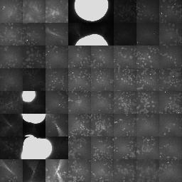
Here we show you the errors which arise from using low quality images for measurement and improper manipulation of thresholds for segmentation.
The segmentation of these images, in all but the first, is done on the dark part of the image, to simulate a darkening sample staining on a brighter background.

Threshold manipulation induces artefacts

A movie sequence (linked with histogram) which illustrates the changes (decrease) in object size with increasing threshold. The threshold changes from 0 tot 255 in this 256-level (8-bit) gray image.
In the graph the red line shows the number of detected objects at a given threshold, the green line the average area (x10) and finally the blue line the total area (x1000). The average area is shown from a threshold of 40 and higher.
This graph illustrates the changes that occur as a result of an increasing threshold in this high contrast image, the resulting objects change in shape and size and as such also the resulting feature measurements. The change is minimal only in the intermediate greylevels. This case illustrates the importance of a reproduceable image segementation.
The image histogram predicts the influence of different threshold settings on the resulting data.

Uneven staining of the entire cell introduces artefacts

In the graph the cyan line shows the number of detected objects at a given threshold and the blue line the total area (x1000).
The graph illustrates the changes that occur as a result of an increasing threshold in this image of a stellate cell, the resulting object changes in shape and size and as such also the resulting feature measurements. Up to a certain level the counting of the number of cells is insensitive to a change of the threshold in contrast to the area measurement which changes at each threshold level.
The image histogram predicts the influence of different threshold settings on the resulting data.

Uneven staining of the offshoots only, introduces artefacts

In the graph the cyan line shows the number of detected objects at a given threshold and the blue line the total area (x1000).
In this image only the offshoots are uneven stained. The graph illustrates the changes that occur as a result of an increasing threshold in this image of a stellate cell. Up from a certain threshold the resulting object changes in shape and size and as such also the resulting feature measurements.
Up to a certain level the counting of the number of cells is insensitive to a change of the threshold and in this case also the area measurement which starts changing when the offshoots appear in the segmented object.
The image histogram predicts the influence of different threshold settings on the resulting data.

Maximum contrast image

The image on the left shows an artificial maximum contrast image, containing only black (greylevel 0) and white (greylevel 255), as shown in the histogram.
The graph illustrates the result of using different threshold levels for segmentation of this image and the result on the total area detected.
Changing the threshold in the intermediate greylevels (1 to 254) has no effect on the total area.
The image histogram predicts the influence of different threshold settings on the resulting data.

Minimum contrast image

The image on the left shows an artificial image with no contrast, there is a gradual change of greylevels from black (greylevel 0) to white (greylevel 255). The histogram shows a uniform distribution of greylevels.
The graph illustrates the result of using different threshold levels for segmentation of this image and the result on the total area detected.
Changing the threshold in the intermediate greylevels (1 to 254) has a dramatic effect on the total area detected.
The image histogram predicts the influence of different threshold settings on the resulting data.

Gradual greylevel difference image

The image on the left shows an artificial image with a gradual change of greylevels in the intermediate part of the image from black (greylevel 0) to white (greylevel 255). There is no intermediate level suitable for setting a threshold, every small change oft he threshold results is an other total area measurement.
The graph illustrates the result of using different threshold levels for segmentation of this image and the result on the total area detected.
Changing the threshold in the intermediate greylevels (1 to 254) has a dramatic effect on the total area detected.
The image histogram predicts the influence of different threshold settings on the resulting data.

Intermediate contrast image

The image on the left shows an artificial image with intermediate contrast, there is a gradual change of greylevels in the dark part of the image from black (greylevel 0) to dark grey (greylevel 67). The bright part of the image goes from light grey (greylevel 179) to white (greylevel 255). The histogram shows a double flat distribution of greylevels, with nothing in between.
The graph illustrates the result of using different threshold levels for segmentation of this image and the result on the total area detected.
Changing the threshold in the intermediate greylevels (68 to 178) has no effect on the total area detected, as there is a broad gap in the image histogram.
The image histogram predicts the influence of different threshold settings on the resulting data.

III. Dark current and ratio measurement

Dark current subtraction

The image on the left shows two spots with an intensity of 200 and 100 respectively. The image on the right shows the same spots, but with a dark current level of 50.
The ratio calculated from the first image: 200/100=2, the second ratio however shows a decrease of 33 percent compared to the first: 250/150=1.67 .
Subtraction of the dark current in the second image yields the same result as in the first: (250-50)/(150-50)=2.
For ratio measurements it is important to subtract the dark current before calculating the ratio.

Acknowledgments

I am indebted, for their pioneering work on automated digital microscopy and High Content Screening (HCS) (1988-2001), to my former colleagues at Janssen Pharmaceutica (1997-2001 CE), such as Frans Cornelissen, Hugo Geerts, Jan-Mark Geusebroek and Roger Nuyens, Rony Nuydens, Luk Ver Donck, Johan Geysen and their colleagues.

Many thanks also to the pioneers of Nanovid microscopy at Janssen Pharmaceutica, Marc De Brabander, Jan De Mey, Hugo Geerts, Marc Moeremans, Rony Nuydens and their colleagues. I also want to thank all those scientists who have helped me with general information and articles.

The author of this webpage is Peter Van Osta.
Private email: pvosta at gmail dot com

Back to homepage