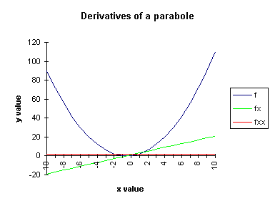
A parabole y=x2+x and its first (fx=2*x+1) and second order (fxx=2) derivatives.
Differential geometry is geometry done using differential calculus or shape description through derivatives. It applies techniques from multivariable calculus and linear algebra to study features of curves and surfaces of dimension 1, 2, and higher. Although this article is limited to 2D, the differential geometry approach can be used for 1D, 2D, 3D and 4D signal and image processing and the digital elevation models (DEM) of geomorphometry. The basic principle is "what you describe is what you get".
This webpage gives an overview grayscale scale space or differential geometry as it
can be used in digital image processing, from digital microscopy and
High Content Screening (HCS) to
medical imaging, geology, and astronomy or any other spatial and temporal structure in a dynamic space-time continuum.
The geometric properties of differential gray-value invariants allow for the
selection of structural image features for analysis and quantification. Although this article is limited to 2D,
the scale space approach can be used for 3D and even 4D image processing. Scalespace stacks (dimension, scale, order) can also
be used in convolutional neural networks, such as in the
M5 framework for exploring the cytome.
The basic principle is "what you describe is what you get".
For an introduction to the spatial color model see
color scale space, which is another application
of scale space applied to color image processing in microscopy and High Content Screening.
This webpage was inspired by the pioneering work on High Content Screening and microscopy at the now defunct Biological Imaging laboratory (BIL) at Janssen Pharmaceutica in Beerse (Belgium).
The principal interpretations of derivatives of a function f concern instantaneous rate
of change and tangency.
In mathematics the derivatives of a one-dimensional function f are denoted as:
fx=dy/dx = 1st order derivative (the slope of the
function)
fxx=d2y/dx2 = 2nd order derivative
(the curvature of the function, or the rate of change of the slope)
fxxx=d3y/dx3 = 3rd order derivative
(the rate of change of the curvature of the function)
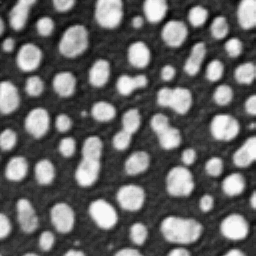
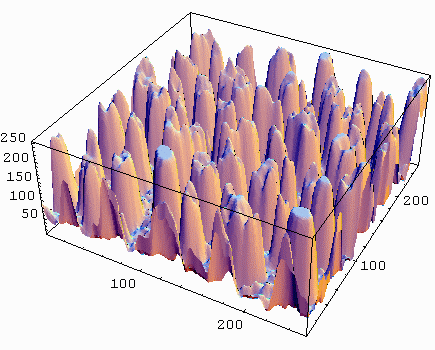
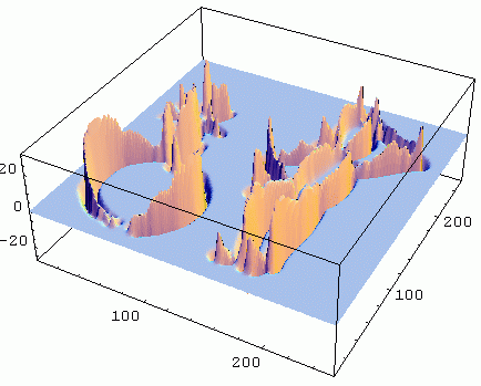
A gray scale 2D image and the gray values (intensities) plotted in a 3D view. The x,y axis is the
position of the pixel in the 2D plane of the image, while the z-axis is the gray value
or intensity of the pixel.
A 2D image can be visualized as a 3D landscape by plotting the surface height proportional to
the pixel gray value. The principles of differential geometry can be used on 2D images, which becomes clear if we plot
the intensity profile of the image in 3D view.
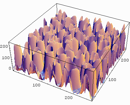
The intensity profile of the image constitutes a landscape of (dark) valleys and
(bright) hills and ridges, which form the curves of a 2D function. The concepts of image processing become similar to the concepts
being used in terrain analysis. Terrain analysis employs elevation data to describe the landscape, for basic visualization, modeling,
or to support decision making.
Geomorphometry
is 'the science of quantitative land surface analysis or topographic quantification; its operational focus is the extraction of
land-surface parameters and objects from digital elevation models (DEM)'
(see Geomorphometry: Concepts, Software, Applications, Tomislav Hengl, Hannes I. Reuter, Elsevier, 2009, p. 4).
Digital elevation models resemble a 3D plot of the intensity profile of a 2D image, which makes studying the intensity profile of an image
similar to studying the topography of a terrain.
The basic notions of geomorphometry and scale space consist of concepts such as:
The 3D luminance profile of a 2D image (L) can be seen as a luminance landscape. L(x, y) is the luminance function (pixel values) of an image and the first order derivative with respect to x is Lx, and the derivative with respect to y is Ly. The geometric interpretation of the first order derivative or gradient at x0 is the slope of the tangent line to the curve at point x0: slope = Δy/Δx. The first derivative tells us how whether a function is increasing or decreasing, and by how much it is increasing or decreasing. The second derivative (curvature or concavity) with respect to x is Lxx, the second derivative with respect to y is Lyy.
Besides using a Cartesian coordinate system
we can also use gauge coordinates such as the gradient or curvature gauge.
Gauge coordinates are coordinates with respect to axes that are attached to the function geometry.
A gauge coordinate system therefore is independent of the natural coordinate axes.
The differentiation of the 2D image is done by
convolving the original image
with the derivatives of a 2D Gaussian kernel or, equivalently, by multiplying the
Fourier transform
of the original image with the Fourier transform of the Gaussian
and doing the reverse Fourier transform of the result.
The same principles can be extended to 3D images, but this is beyond the current scope of this webpage. The principles of differential geometry can also be used for the analysis of spacetime phenomena, but this is also beyond the scope of this article.
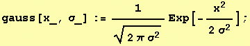
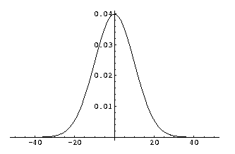
1D Gaussian, probability density function (PDF)
of the normal distribution with
standard deviation σ and
variance σ2
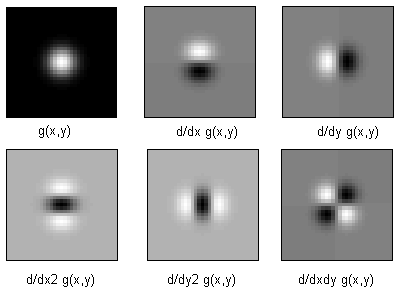
2D Gaussian kernels,
up to 2nd order derivatives, bivariate normal distribution and equal standard deviation σ =σx=σy
The Gaussian kernel is the unique kernel for differentiation for an uncommitted front-end (eg. human eye). Scale-space uses the Gaussian function and its derivatives as a physical differential operator. In computational vision we replace the mathematical derivatives by fuzzy derivatives or Gaussian Derivatives. Differentiating an image is done by convolving the image in the spatial domain with a Gaussian kernel with a standard deviation σ. An alternative way is using the Fourier transform of a convolution, which is the pointwise product of Fourier transforms of the image and the Gaussian kernel. In other words, convolution in one domain (e.g., spatial domain) equals point-wise multiplication in the other domain (e.g., frequency domain) (see convolution theorem). The Gaussian kernel we will use here is isotropic, which means that the behavior of the function is in any direction the same. For 2D this means the Gaussian function is circular, for 3D it would look like a fuzzy sphere. When we would use unequal standard deviations in the different dimensions we would apply an anisotropic Gaussian kernel. The σ (sigma) parameter of the Gaussian kernel determines the size (scale) of the features that are resolved, ie. it is a measure for the aperture of the filter. Local image observations with Gaussian Derivatives are always done at a finite scale (σ) to be selected by the observer. The larger you make the standard deviation σ of the Gaussian kernel, the more the image gets blurred. In order to find the optimal size of the Gaussian filter we may apply many filters of different sizes and embed them in a structure called a (Gaussian) scale space pyramid. An exponential increase in scale was proposed by Koenderink in 1984 and a method for automatic scale detection was proposed by Lindeberg in 1998.
L is the image
L(x, y) is the luminance function (pixel values) of a 2D image
Lx = 1st order x derivative
Ly = 1st order y derivative
Lxx = 2nd order x derivative, etc.
Li = 1st order Partial Differential Equation
(PDE) according to summation convention
"i" sums over all dimensions, i.e. Li = Lx+Ly
Li is a vector:{Lx,Ly,Lz}. Summation convention on paired indices
Lii = 2nd order, Lii = Lxx+Lyy
Lij = 2nd order, Lij = Hessian matrix
The classical Euclidean image coordinate frame is an arbitrary convenient choice without much relevance. Attaching the coordinate frame to the local image structure makes the coordinate frame independent of arbitrary Euclidean transformations (rotations, scalings and translations).
The most important gauge coordinate systems are:
Zero order derivative of a 1D Gaussian kernel, sigma (σ) is 10.0.
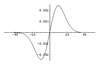
First order derivative of a 1D Gaussian kernel, sigma (σ) is 10.0.
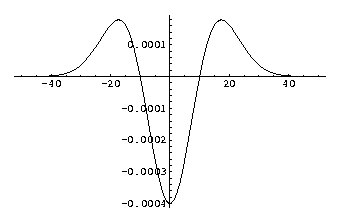
Second order derivative of a Gaussian kernel, sigma (σ) is 10.0.
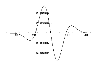
Third order derivative of a 1D Gaussian kernel, sigma (σ) is 10.0
Convolving an image with a Gaussian kernel and derivatives of the Gaussian kernel, highlights
features of the image with a size larger than the chosen scale sigma (σ).
The examples shown here are for 2D images, but can be extended to 3D (spatial), 4D (spatiotemporal)
and spatiospectral dimensions.

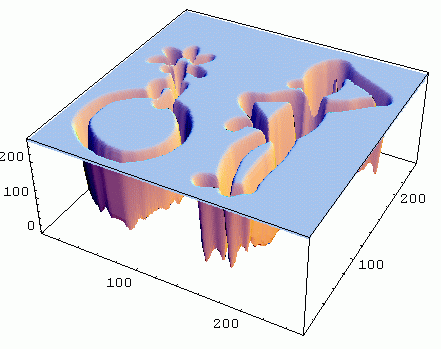
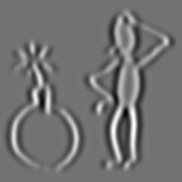
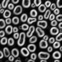
The original 256x256 pixels image L(x, y) from which the following differentiated images are derived.

Zero order Gaussian derivative in x and y direction (Lxy), just blurs the image. Sigma (σ, scale) is 2.
Original resolution is 2562

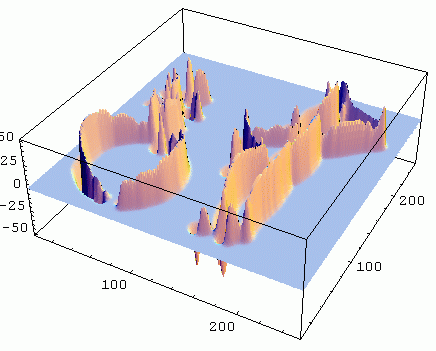
First order Gaussian derivative in x direction (Lx). Sigma (σ, scale) is 2.
Second order Gaussian derivative in x direction (Lxx). Sigma (σ, scale) is 2.
Invariant differential feature detectors are polynomial combinations of image derivatives, which exhibit invariance under some chosen group of transformations.
The image on the left shows the response intensity of the Canny filter (bright means
high gradient strength), which is also shown in 3D on the right, the scale, sigma (σ), is 3.
Intensity gradient = Canny edge detector
= ||∇L|| = Lw
For an explanation of Lv, Lw, etc. see the section on gauge coordinates.
Second order derivatives yield isophote and flowline curvature and cornerness of an image. Isophotes are lines drawn through areas of constant brightness while flowlines are lines drawn through areas of changing brightness.
Gradient2 = LiLi = Lx2 + Ly2
Marr edge detector = ∇2L
= Lxx + Lyy
Canny edge detector = Lww ≈ 0
Laplacian of Gaussian
= Trace of Hessian matrix = trHf = Lii = Lxx + Lyy
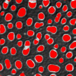
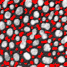
Determinant of the Hessian matrix
(blob detection) = |Hf| = LxxLyy-Lxy2
Euclidian shortening flow = Lvv = Ls
Ridge strength = Lvv
Derivative of gradient in gradient direction = Lww (if Lww=0, Lw maximal)
Deviation from flatness = D = Sqrt(tr H2) = Sqrt(LijLji) =
Sqrt(Lxx2 + 2Lxy2 + Lyy2)
Isophote curvature = K = -Lvv / Lw
Flow-line curvature = -Lvw / Lw
Isophote density per unit luminance = -Lww / Lw
Principal intensity surface curvature in principal coordinates in 2D:
Kp1 = Lxx/Sqrt(Lx2 + Ly2)
Kp2 = Lyy/Sqrt(Lx2 + Ly2)
Inflexion strength = LvvLw5-3LvvLvwLw4
Umbilicity = U = (trH)2/TrH2 - 1 = (Lxx + Lyy)2 / D2 = Lll2 / LijLji
Elongatedness = E = ((trH)2(2trH2-(trH)2))/(2trH2)2 = (Lxx2 + Lyy2)/D4
Third order derivatives provide T-junction detection. T-junctions in an image occur at occlusion points which occur at a point where a contour ends or emerges because there is another object in front of the contour.
T-junction = ((LvvLvvLvwLvw+LvvLvvLwwLww)/Lw2-2LvvLvvvLvw/Lw-2LvvLvvwLww/Lw+(LvvvLvvv+LvvwLvvw))/Lw2
All resultants and discriminants are Euclidian and affine invariant
R12 = Corner strength = Lx2Lyy-2LyLxLxy+ Ly2Lxx = LvvLw2
D1 = 1
D2 = detH = -Lxy2+Lyy + Lxx or
Lxx+Lyy-Lxy2
A partial differential equation (PDE) is a differential equation that contains unknown multivariable functions and their partial derivatives. PDEs can be used to describe a wide variety of phenomena in multidimensional systems such as images.
Lx = 0
Ly = 0
LxxLyy-Lxy2 >= 0
|Lxx| > threshold
threshold determines salient features
Lx = 0
Ly = 0
LxxLyy-Lxy2 >= 0
Lxx < -threshold
threshold determines salient features
Lx = 0
Ly = 0
LxxLyy-Lxy2 >= 0
Lxx > threshold
threshold determines salient features
Lx = 0
Ly = 0
LxxLyy-Lxy2 < 0
Lx = 0
Ly = 0
LxxLyy-Lxy2 = 0
affine corner detection: LwwLw2
with high curvature: LwwLw2 > threshold
Bright ridges: Lqq < -4.0 * threshold / sigma2
Dark ridges: Lpp > 4.0 * threshold / sigma2
threshold determines salient features
A convenient way to calculate features invariant under Euclidean coordinate transformations is done by using gauge coordinates such as the gradient or curvature gauge. Any combination of derivatives with respect to gauge coordinates is invariant under Euclidean transformations.
Coordinate axes in space can be chosen arbitrarily. The space and its properties
do not change when we change the coordinate axes. But if coordinate systems are
arbitrary, what then is the value of derivatives in the axis direction?
The individual derivatives
(fx, fxy, ...) are of no use. It is the collection of all
derivatives in the N-jet (collection of all spatial image derivatives
up to order N) that are of importance as it has geometrical meaning
independent of the arbitrary coordinate system.
Gauge coordinates are coordinates with respect to axes that are attached to
the function geometry. A gauge coordinate system therefore is independent of
the natural coordinate axes.
Examples of gauge systems are the gradient gauge and the
principal curvature gauge, in which all points in the image have their
own gauge coordinate system attached to it.
The word gauge (in gauge theory) was introduced as the German word maßstab by Hermann Weyl (1885-1955 CE). In 1918, he introduced the notion of gauge, and gave the first example of what is now known as a gauge theory.
The classical Euclidean image coordinate frame is an arbitrary convenient choice.
Attaching the coordinate frame to the local image structure makes the coordinate frame independent of arbitrary
Euclidean transformations (rotations, scalings and translations).
The most important gauge coordinate systems are:
Gradient gauge coordinates, where w is the coordinate in the gradient direction (flowline, maximal change of the intensity)
and v is the coordinate perpendicular to the gradient direction (isophote).
A gauge is a "coordinate system" that varies depending on one's "location" with respect to some "base space" or
"parameter space", a gauge transform is a change of coordinates applied to each such location, and a
gauge theory is a
model for some physical or mathematical system to which gauge transforms can be applied (and is typically gauge invariant,
in that all physically meaningful quantities are left unchanged (or transform naturally) under gauge transformations).
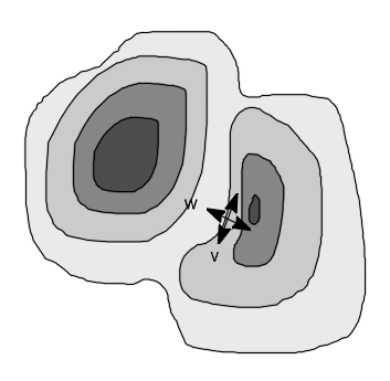
Consider intrinsic geometry: every point is described in such a way, that if we have the same structure,
or local landscape form, no matter the rotation, the description is always the same.
This can be accomplished by setting up in each point a dedicated coordinate frame which is determined by
some special local directions given by the landscape locally itself.
In each point separately the local coordinate frame is fixed in such a way that one frame vector points
to the direction of maximal change of the intensity, and the other perpendicular to it (90 degrees clockwise).
We can now fix locally the direction for our new intrinsic local coordinate frame (v and w in the image) and
this set of local directions is called a gauge, the new frame forms the gauge coordinates.
A special notation is used in image processing for this gauge system: the w,v-coordinates. w is the coordinate in the gradient direction (maximal change of the intensity) and v is the coordinate perpendicular to the gradient direction.
{v,w} are gradient gauge coordinates, w along and v perpendicular on the gradient;
w and v are unit vectors. Lw is the derivative of the luminance field in the w
direction.
Lv = 0, Lw = |Grad L|
Lvv, Lwv, Lww = 2nd order, etc.
Lww is also called the SDGD (Second Derivative in Gradient Direction).
Lw gives us information about the local change in intensity of an
image, which is a first order derivative phenomenon.
In situations where the gradient gauge vanishes (Lx=0, Ly=0), the second order differentials may indicate that something interesting is happening, for instance the points along the axis of a line. A gauge system suitable for this phenomenon is the curvature gauge. The eigenvectors of the Hessian matrix HL then provide a powerful way of defining a gauge system.
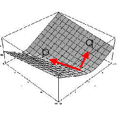
The local second order differentials around a point in a 2D image can be grouped into a Hessian matrix in which all second order derivatives are gathered, it describes the local second-order profile of intensity variations in a 2D image.
![]()
The partial second order derivatives of a 2D image L(x,y) are represented
like Lxx, Lxy, etc. .
The Hessian matrix of second order derivatives is a symmetric matrix and can be
transformed to a diagonal matrix, using a rotation matrix. The coordinate frame
that diagonalizes the Hessian matrix is often denoted as the (p,q)-frame, it is
built from the eigenvectors of the Hessian matrix.
The eigenvectors of the Hessian, p and q, point in the directions of the
minimal and maximal directional second order derivatives.
The eigenvalues of the Hessian are the second order differentials
fpp and fqq or Lpp and Lqq.
{p,q} are the Hessian gauge coordinates, this diagonalizes the Hessian
(eigenvalues of the Hessian matrix), by definition Lpq = 0
The trace (trHf) of a matrix equals the sum of its diagonal elements,
it is a sort of Laplacian, it might be called the
mean curvature and it describes the curvature at patch boundaries.
The sign of the trace indicates whether creases are ridges or valleys
and its magnitude reflects the angle at which two linear patches meet.
The trace of the Hessian=trHf=fxx+fyy=
Lxx+Lyy=Lww+Lvv
The determinant (|Hf|) of the Hessian matrix is:
|Hf|=fxxfyy-fxy2=
LxxLyy-Lxy2=LwwLvv-Lvw2
The determinant is sometimes called deviation of flatness, and it indicates the overall change in first-order information; magnitude and direction.
The term Hessian was coined by James Joseph Sylvester (1814-1897 CE), named for Otto Hesse (1811-1874 CE), who had used the term functional determinants.
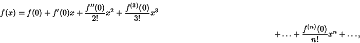
Locally an image is characterized with its Taylor expansion. A way to approximate an image is to perform a Taylor expansion of the local image structure. Locally, i.e. in a small neighborhood of a point, an image (as any function) can be represented by its Taylor expansion. A Taylor series is a series expansion of a function, it is the most basic tool for approximation of functions. It is a representation of a function as an infinite sum of terms that are calculated from the values of the function's derivatives at a single point.
A Taylor expansion is useful for calculating image values between pixels and extrapolation.
Truncating the Taylor expansion at some finite number N, we obtain an approximated
representation of the function (image). Since the complete expansion (N=infinity)
is a unique description of the function f, the approximated expansion can
be the same for different images.
The local N-jet is definded as the complete set of images which all give the
same Taylor expansion at that point up to order N. This is the set of images
which are equal in the first N derivatives at that point.
The scale has be to taken into account in the Taylor-expansion, The scale is the
level of resolution at which we look at an image, only resolving features at a certain
level of resolution (the aperture of the filter in image analysis). All derivatives
are scaled derivatives.
Consider a one-dimensional function f(x) that is smooth - when we say 'smooth', what we mean is that its derivatives exist and are bounded (for the following discussion, we need f to have (n+1)derivatives). We would like to approximate f(x) near the point x=a, and we can do it as follows with a 1-D Taylor series:
If we look at the infinite sum (let n-> infinity), then
the resulting infinite sum is called the Taylor series of f(x) about x=a.
This result is also know as
Taylor's Theorem.
If a=0, the expansion is known as a Maclaurin series, which is a Taylor series expansion of a function about 0. The third order Taylor expansion (and beyond) becomes:
An alternative form of the 1-D Taylor series may be obtained by letting
![]()
so that
![]()
Substitute this result into () to give
![]()
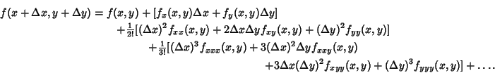
We want to generalize Taylor expansions to functions of more than one variable so we can use it in image processing and analysis. Our approach will be limited to 2D images, but can be expanded to 3D images also. Let us consider a two-dimensional function f(x, y). We want to approximate f(x0+Δx, y0+Δy) for Δx and Δy near zero. We rewrite f(x0+Δx, y0+Δy) = F(1) as F(t) = f(x0+tΔx, y0+tΔy) where x0, y0, Δx and Δy are constants, so that F is now a function of a single variable t. Now we can use out single variable formula with t0=0 and Δt=1 (e.g. Maclaurin series). For this we need to compute various derivatives of F(t) at t = 0, by applying the chain rule to our formula.
A Taylor series of a function in two variables f(x,y), such as a 2D-image, can be given by expanding f(x+Δx, y+Δy):
Let us now take this step by step. Given ")


First, we rewrite Δx as α0 and Δy as α1 and parameterise:
 = x_0 + \alpha_0 t")
 = y_0 + \alpha_1 t")
Then, because Δx, Δy, α0 and α1 are constants, we now have a function of a single variable t:
 = f(x(t), y(t)) = f(t)")
The Taylor series expansion of ")

 = f(0) + t f'(0) + \dfrac{t^2}{2} f''(0) + ...")
Applying the chain rule we get:

 = \dfrac{\partial}{\partial x} \left ( \alpha_0 \dfrac{\partial f}{\partial x} + \alpha_1 \dfrac{\partial f}{\partial y} \right ) \dfrac{dx}{dt} + \dfrac{\partial}{\partial y} \left (\alpha_0 \dfrac{\partial f}{\partial x} + \alpha_1 \dfrac{\partial f}{\partial y} \right )\dfrac{dy}{dt} = \alpha_0^2 \dfrac{\partial^2 f}{\partial x^2} + 2 \alpha_0 \alpha_1 \dfrac{\partial^2 f}{\partial x \partial y} + \alpha_1^2 \dfrac{\partial^2 f}{\partial y^2}")
Substituting this in the Taylor expansion gives:
![f(t) = f(0) + t \alpha_0 \dfrac{\partial f}{\partial x} + t \alpha_1 \dfrac{\partial f}{\partial y} + \dfrac{1}{2} \left [ \alpha_0^2 t^2 \dfrac{\partial^2 f}{\partial x^2} + 2 \alpha_0 \alpha_1 t^2 \dfrac{\partial^2 t}{\partial x \partial y} + \alpha_1^2 t^2 \dfrac{\partial^2 f}{\partial y^2} \right ] + ...](https://s0.wp.com/latex.php?latex=f%28t%29+%3D+f%280%29+%2B+t+%5Calpha_0+%5Cdfrac%7B%5Cpartial+f%7D%7B%5Cpartial+x%7D+%2B+t+%5Calpha_1+%5Cdfrac%7B%5Cpartial+f%7D%7B%5Cpartial+y%7D+%2B+%5Cdfrac%7B1%7D%7B2%7D+%5Cleft+%5B+%5Calpha_0%5E2+t%5E2+%5Cdfrac%7B%5Cpartial%5E2+f%7D%7B%5Cpartial+x%5E2%7D+%2B+2+%5Calpha_0+%5Calpha_1+t%5E2+%5Cdfrac%7B%5Cpartial%5E2+t%7D%7B%5Cpartial+x+%5Cpartial+y%7D+%2B+%5Calpha_1%5E2+t%5E2+%5Cdfrac%7B%5Cpartial%5E2+f%7D%7B%5Cpartial+y%5E2%7D+%5Cright+%5D+%2B+...&bg=ffffff&fg=333333&s=0 "f(t) = f(0) + t \alpha_0 \dfrac{\partial f}{\partial x} + t \alpha_1 \dfrac{\partial f}{\partial y} + \dfrac{1}{2} \left [ \alpha_0^2 t^2 \dfrac{\partial^2 f}{\partial x^2} + 2 \alpha_0 \alpha_1 t^2 \dfrac{\partial^2 t}{\partial x \partial y} + \alpha_1^2 t^2 \dfrac{\partial^2 f}{\partial y^2} \right ] + ...")
Since 

![f(t) = f(0) + (x- x_0) \dfrac{\partial f}{\partial x} + (y - y_0) \dfrac{\partial f}{\partial y} + \dfrac{1}{2} \left [ (x - x_0)^2 \dfrac{\partial^2 f}{\partial x^2} + 2 (x - x_0)(y - y_0) \dfrac{\partial^2 f}{\partial x \partial y} + (y - y_0)^2 \dfrac{\partial^2 f}{\partial y^2} \right ] + ...](https://s0.wp.com/latex.php?latex=f%28t%29+%3D+f%280%29+%2B+%28x-+x_0%29+%5Cdfrac%7B%5Cpartial+f%7D%7B%5Cpartial+x%7D+%2B+%28y+-+y_0%29+%5Cdfrac%7B%5Cpartial+f%7D%7B%5Cpartial+y%7D+%2B+%5Cdfrac%7B1%7D%7B2%7D+%5Cleft+%5B+%28x+-+x_0%29%5E2+%5Cdfrac%7B%5Cpartial%5E2+f%7D%7B%5Cpartial+x%5E2%7D+%2B+2+%28x+-+x_0%29%28y+-+y_0%29+%5Cdfrac%7B%5Cpartial%5E2+f%7D%7B%5Cpartial+x+%5Cpartial+y%7D+%2B+%28y+-+y_0%29%5E2+%5Cdfrac%7B%5Cpartial%5E2+f%7D%7B%5Cpartial+y%5E2%7D+%5Cright+%5D+%2B+...&bg=ffffff&fg=333333&s=0 "f(t) = f(0) + (x- x_0) \dfrac{\partial f}{\partial x} + (y - y_0) \dfrac{\partial f}{\partial y} + \dfrac{1}{2} \left [ (x - x_0)^2 \dfrac{\partial^2 f}{\partial x^2} + 2 (x - x_0)(y - y_0) \dfrac{\partial^2 f}{\partial x \partial y} + (y - y_0)^2 \dfrac{\partial^2 f}{\partial y^2} \right ] + ...")
and finally:
![f(x, y) = f(x_0, y_0) + (x- x_0) \dfrac{\partial f}{\partial x} + (y - y_0) \dfrac{\partial f}{\partial y} + \dfrac{1}{2} \left [ (x - x_0)^2 \dfrac{\partial^2 f}{\partial x^2} + 2 (x - x_0)(y - y_0) \dfrac{\partial^2 f}{\partial x \partial y} + (y - y_0)^2 \dfrac{\partial^2 f}{\partial y^2} \right ] + ...](https://s0.wp.com/latex.php?latex=f%28x%2C+y%29+%3D+f%28x_0%2C+y_0%29+%2B+%28x-+x_0%29+%5Cdfrac%7B%5Cpartial+f%7D%7B%5Cpartial+x%7D+%2B+%28y+-+y_0%29+%5Cdfrac%7B%5Cpartial+f%7D%7B%5Cpartial+y%7D+%2B+%5Cdfrac%7B1%7D%7B2%7D+%5Cleft+%5B+%28x+-+x_0%29%5E2+%5Cdfrac%7B%5Cpartial%5E2+f%7D%7B%5Cpartial+x%5E2%7D+%2B+2+%28x+-+x_0%29%28y+-+y_0%29+%5Cdfrac%7B%5Cpartial%5E2+f%7D%7B%5Cpartial+x+%5Cpartial+y%7D+%2B+%28y+-+y_0%29%5E2+%5Cdfrac%7B%5Cpartial%5E2+f%7D%7B%5Cpartial+y%5E2%7D+%5Cright+%5D+%2B+...&bg=ffffff&fg=333333&s=0 "f(x, y) = f(x_0, y_0) + (x- x_0) \dfrac{\partial f}{\partial x} + (y - y_0) \dfrac{\partial f}{\partial y} + \dfrac{1}{2} \left [ (x - x_0)^2 \dfrac{\partial^2 f}{\partial x^2} + 2 (x - x_0)(y - y_0) \dfrac{\partial^2 f}{\partial x \partial y} + (y - y_0)^2 \dfrac{\partial^2 f}{\partial y^2} \right ] + ...")
A Taylor series approximates continuous functions by using derivative information of different orders and in the same way the image intensity function of an image could be approximated. By using diferent orders of derivatives all possible shapes of the image could be classified and detected. The Taylor approximation is being done by fitting a polynomial to the pixel intensities in a patch or region of the image. By using a "sliding window" algorithm for patch-based operations we try to determine the fit with the Taylor expansion up to the nth order. At each postion of the sliding window we assign the polynomial's derivatives to the pixel at the window's center. The window slides over the entire image, thereby creating a new intensity plot proportional to the response of the polynomial to each patch in the image. The aperture of the Gaussian filter defines the size of the patch and determines the size of the features which will be detected. Keep in mind, this approach can also be used for higher dimensional spatial and spatiotemporal data.
A necessary condition that a function f assumes a relative maximum or a
relative minimum at (x0, y0) is that:
fx = fy = 0 at (x0,y0)
If this condition is true then in summary the following criteria can be used.
All subsequent images were analyzed with sigma (σ)= 5.0.
fx = 0, fy = 0 and fxxfyy > f2xy
or i.o.w.
fx = 0, fy = 0 and fxxfyy - f2xy > 0
or i.o.w.
Lx = 0, Ly = 0 and LxxLyy - Lxy2 > 0
fx = 0, fy = 0 and fxxfyy < f2xy
or i.o.w.
fx = 0, fy = 0 and fxxfyy - f2xy < 0
or i.o.w.
Lx = 0, Ly = 0 and LxxLyy - Lxy2 < 0
fx = 0, fy = 0 and fxxfyy = f2xy
or i.o.w.
fx = 0, fy = 0 and fxxfyy - f2xy = 0
or i.o.w.
Lx = 0, Ly = 0 and LxxLyy - Lxy2 = 0
fxx < 0 and fxxfyy > f2xy
or i.o.w.
fxx < 0 and fxxfyy - f2xy > 0
or i.o.w.
Lxx < 0 and LxxLyy - Lxy2 > 0
or i.o.w.
Lww < 0 and LvvLww - Lvw2 > 0
fxx > 0, fxxfyy > f2xy
or i.o.w.
fxx > 0, fxxfyy - f2xy > 0
or i.o.w.
Lxx > 0 and LxxLyy - Lxy2 > 0
or i.o.w.
Lww > 0, LvvLww - Lvw2 > 0
fxxfyy < f2xy
or i.o.w.
fxxfyy - f2xy < 0
or i.o.w.
LxxLyy - Lxy2 < 0
or i.o.w.
LvvLww - Lvw2 < 0
By using for instance Lxx/L in the above mentioned equations, a normalisation relative to the
image intensity is obtained.
By selecting for instance Lxx/L > Threshold or Lxx/L < Threshold, a noise
reduction is performed, as only salient features are selected.
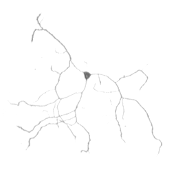
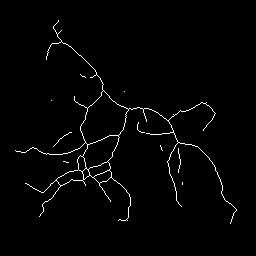
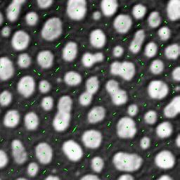
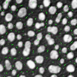
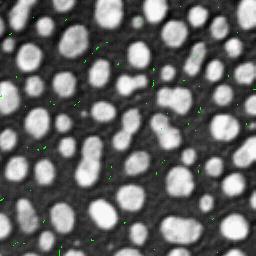
Tracing the neurites of a neuron (left) with differential geometry as an example of a line detector (result on the right).
The equation used for detecting a dark ridge, with sigma (σ)=2.0 and threshold 1.0:
Lpp > 4.0 * threshold / σ2
The purpose of a line filter is the discrimination of line structures from other
image structures.
A line or a bar is a second order differential structure (see Hessian matrix).
The points along the axis have a gradient near zero. A gauge system that is capable of
capturing these local phenomena is the above mentioned principal curvature gauge.
As we have seen, the eigenvectors of the Hessian matrix, p and q, point in the
directions of the minimal and maximal directional second order derivatives.
The difference between Lqq and Lpp determines the directionality of
the local image structure.
If Lqq = Lpp, there is no preferred orientation;
if Lqq >> Lpp this indicates a line structure.
In short, we have a line when Lqq - Lpp > Th and Lx = 0, Ly = 0. The
parameter Th determines the saliency of the line (see also C. Steger (1998)).
The larger the difference between the trace of the Hessian (trHf) and the determinant (|Hf|), the larger is the directionality of the local 2D image structure and as such the probability for a line.
With respect to the Cartesian coordinate frame (x,y):
p = (fxx-fyy- sqrt((trHf)2-4*|Hf|)) / (2*fxy)
q = (fxx-fyy+ sqrt((trHf)2-4*|Hf|)) / (2*fxy)
or in L notation:p = (Lxx-Lyy- sqrt((trHf)2-4*|Hf|)) / (2*Lxy)
q = (Lxx-Lyy+ sqrt((trHf)2-4*|Hf|)) / (2*Lxy)
The eigenvalues of the Hessian, expressed as a function of the
trace (trHf) and the determinant (|Hf|)
of the Hessian matrix:
Lpp = 0.5*(trHf-
sqrt((trHf)2-4*|Hf|))
Lqq = 0.5*(trHf+ sqrt((trHf)2-4*|Hf|))
The eigenvalues of the Hessian matrix in L notation, expressed in Cartesian coordinates:
Lpp = 0.5*(Lyy+Lxx-
sqrt((Lyy+Lxx)2-4*(LyyLxx-Lyx2)))
Lqq = 0.5*(Lyy+Lxx+ sqrt((Lyy+Lxx)2-4*(LyyLxx-Lyx2)))
The eigenvalues of the Hessian matrix in L notation expressed in gauge coordinates:
Lpp = 0.5*(Lww+Lvv-
sqrt((Lww+Lvv)2-4*(LwwLvv-Lvw2)))
Lqq = 0.5*(Lww+Lvv+ sqrt((Lww+Lvv)2-4*(LwwLvv-Lvw2)))
For additional information you may also contact my former colleague Jan-Mark Geusebroek (UvA) now at Perceptech or Prof. Bart M. ter Haar Romeny (T.U. Eindhoven).
I am indebted, for their pioneering work on automated digital microscopy and High Content Screening (HCS) (1988-2001), to my former colleagues at Janssen Pharmaceutica (1997-2001 CE), such as Frans Cornelissen, Hugo Geerts, Jan-Mark Geusebroek and Roger Nuyens, Rony Nuydens, Luk Ver Donck, Johan Geysen and their colleagues.
Many thanks also to the pioneers of Nanovid microscopy at Janssen Pharmaceutica, Marc De Brabander, Jan De Mey, Hugo Geerts, Marc Moeremans, Rony Nuydens and their colleagues. I also want to thank all those scientists who have helped me with general information and articles.
The author of this webpage is Peter Van Osta.
Private email: pvosta at gmail dot com